On the relatedness between embeddings and dense connections.
the question
Embedding layers are extensively used in language learning and recently we shared results showing improvements in prediction when applying them to sequences of categorical data. There is a nagging question, though, on whether they're really different from dense networks where weights appear to be learned the same way, and whether we avoid any costly operations in most cases.
why embeddings
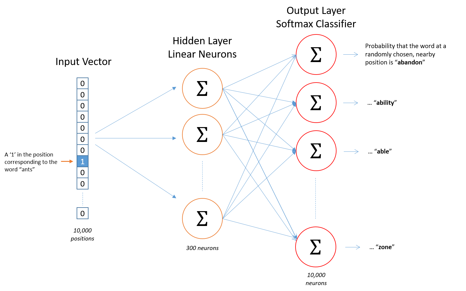
The point of embeddings is simply finding quantitative representations of a large number of categories in their contribution to classification of prediction. For example, in the word representation problem where we want to know what word follows ants in a sentence:
- input is a one-hot vector representing the input word (e.g. ants),
- hidden layer of variable number of dense nodes (the, learned lookup table),
- a softmax layer that forces a probability distribution,
- output is a single vector containing, for every word in our vocabulary, the probability that a randomly selected nearby word is that vocabulary word (e.g. car).
This is outlined in the figure below.
A response on StackOverflow by the user kmario23 provides a good start to defining variables for this post, I've added additional, Tensorflow-specific functions to make this practical. Embedding matrices are typically trained from large (e.g. language) corpora, and are of the shape vocab_size * embedding_dim.
Suppose the following vocabulary:
vocab : ['the','like','between','did','just','national',
		'day','country','under','such','second']
Imagine the following, trained word2vec vectors:
\[ \small{ the : \left( 0.418 0.24968 -0.41242 0.1217 0.34527 -0.044457 -0.49688 -0.17862 \right)}\\ \small{ like : \left( 0.36808 0.20834 -0.22319 0.046283 0.20098 0.27515 -0.77127 -0.76804 \right)}\\ \small{ between : \left( 0.7503 0.71623 -0.27033 0.20059 -0.17008 0.68568 -0.061672 -0.054638 \right)}\\ \small{ did : \left( 0.042523 -0.21172 0.044739 -0.19248 0.26224 0.0043991 -0.88195 0.55184 \right)}\\ \small{ just : \left( 0.17698 0.065221 0.28548 -0.4243 0.7499 -0.14892 -0.66786 0.11788 \right)}\\ \small{ national : \left( -1.1105 0.94945 -0.17078 0.93037 -0.2477 -0.70633 -0.8649 -0.56118 \right)}\\ \small{ day : \left( 0.11626 0.53897 -0.39514 -0.26027 0.57706 -0.79198 -0.88374 0.30119 \right)}\\ \small{ country : \left( -0.13531 0.15485 -0.07309 0.034013 -0.054457 -0.20541 -0.60086 -0.22407 \right)}\\ \small{ under : \left( 0.13721 -0.295 -0.05916 -0.59235 0.02301 0.21884 -0.34254 -0.70213 \right)}\\ \small{ such : \left( 0.61012 0.33512 -0.53499 0.36139 -0.39866 0.70627 -0.18699 -0.77246 \right)}\\ \small{ second : \left( -0.29809 0.28069 0.087102 0.54455 0.70003 0.44778 -0.72565 0.62309 \right)}\\ \]
The embedding matrix is:
emb = np.array([[0.418, 0.24968, -0.41242, 0.1217, 0.34527, -0.044457, -0.49688, -0.17862],
   [0.36808, 0.20834, -0.22319, 0.046283, 0.20098, 0.27515, -0.77127, -0.76804],
   [0.7503, 0.71623, -0.27033, 0.20059, -0.17008, 0.68568, -0.061672, -0.054638],
   [0.042523, -0.21172, 0.044739, -0.19248, 0.26224, 0.0043991, -0.88195, 0.55184],
   [0.17698, 0.065221, 0.28548, -0.4243, 0.7499, -0.14892, -0.66786, 0.11788],
   [-1.1105, 0.94945, -0.17078, 0.93037, -0.2477, -0.70633, -0.8649, -0.56118],
   [0.11626, 0.53897, -0.39514, -0.26027, 0.57706, -0.79198, -0.88374, 0.30119],
   [-0.13531, 0.15485, -0.07309, 0.034013, -0.054457, -0.20541, -0.60086, -0.22407],
   [ 0.13721, -0.295, -0.05916, -0.59235, 0.02301, 0.21884, -0.34254, -0.70213],
   [ 0.61012, 0.33512, -0.53499, 0.36139, -0.39866, 0.70627, -0.18699, -0.77246 ],
   [ -0.29809, 0.28069, 0.087102, 0.54455, 0.70003, 0.44778, -0.72565, 0.62309 ]])


emb.shape
# (11, 8)
We will come back to using emb in exploring how dense layers and embedding layers are related.
weights in vectorized representations
In the example above, and in general, embeddings are simply hidden layer weights. Whether it's the word2vec representations, or the more sophisticated, context-sensitive, representations like ELMo, the goal involves learning a linear combination of layer representations.
Running with the ELMo comparison, the difference in the embeddings from the one derived from the single, hidden layer is in the way we combine hidden layer outputs. The motivation is to combine context-dependent aspects of a word meaning (using higher-level LSTM layer weights), and syntax from lower-level LSTM states in order to represent more information about a token in a single vector.
\[ ELMo_{k}^{\operatorname{task}}=\gamma^{\operatorname{task}} \sum_{j=0}^{L} s_{j}^{\operatorname{task}} \mathbf{h}_{k, j}^{L M} \]
\( \gamma \) acts as a (task-specific) scale to the ELMo vector,
\( s \) are the softmax-normalized weights,
\( k \) is the index of the word of interest,
\( j \) is the index of the layers (total \( L \)) the weighted sum is calculated over,
\( h_{k,j} \) is the output of the \( j \)-th LSTM for the word \( k \).
In summary, we train a multi-layer, bi-directional, LSTM from a large corpus, extract the hidden state of each layer for the input sequence of words, compute a weighted sum of those hidden states to arrive at our final vectorized representation, or embedding. The weight of each hidden state is task-dependent and is learned separately.
using pre-trained embeddings vs. embedding layers
Realated to the overall question of how and why different the results of a study would be using embeddings vs. a fully connected layer, recent work that looked into using task-specific embedding layers or pre-trained embeddings trained on larger text corpora has found intersting results. For embeddings derived from a sufficiently large corpus, we can expect faster training times and lower final loss, from the original author, Meghdad Farahmand:
This can mean that for solving certain NLP tasks, when the training set at hand is sufficiently large (as was the case in the Sentiment Analysis experiments), it is better to use pre-trained word embeddings. But if they are not available, you can still use an embedding layer and expect comparable results. If, however, the training set is small, the above experiments strongly encourage the use of pre-trained word embeddings.
embeddings are simplified, dense layers
In addressing the relation between embeddings and dense layers, I was in search of a clear, functional explanation to why embeddings may be preferred when we have words as input or sequenced, categorical variables over ouputs from dense layers. Coming back to our initialization from before, imagine we want to convert the following sentence to an embedding:
sentence_to_embed = 'like national day'Attempting to use a naive, dense network will need the following process in order to convert this sentence to its vectorized representation:
\[ \text{sentence_to_embed} \rightarrow \text{one hot encoding matrix} \rightarrow \\ \text{matrix multiplication with emb} \]
The Tensorflow process would go something like:
inputs = one_hot(sentence_to_embed)
print(inputs)
# array([[0, 1, 0, 0, 0, 0, 0, 0, 0, 0, 0],
	[0, 0, 0, 0, 0, 1, 0, 0, 0, 0, 0],
	[0, 0, 0, 0, 0, 0, 1, 0, 0, 0, 0]] dtype=float32)

outputs = matmul(inputs, emb)  # kernel matrix
print(outputs)
# array([[0.36808, 0.20834, -0.22319, 0.046283, 0.20098, 0.27515, -0.77127, -0.76804],
       [-1.1105, 0.94945, -0.17078, 0.93037, -0.2477, -0.70633, -0.8649, -0.56118],
       [0.11626, 0.53897, -0.39514, -0.26027, 0.57706, -0.79198, -0.88374, 0.30119]], dtype=float32)
There's a problem here: the inputs size increases dramatically with language size. The embedding layer performs a shortcut: it looks up the index of the words in sentence_to_embed and references the relevant rows of emb to avoid the dot product:
outputs = tf.gather(emb, sentence_to_embed)
# same output as above
That's it for the difference. Embedding layers are limited dense layers, with two limitations: the inputs need to be integers, and you cannot use the bias or activation aspects of dense layers - only the kernel.
takeaway
An embedding layer is a limited version of a dense layer. It is useful to speed up training and to yeild lower final loss, because it avoids costly matrix multiplication through the assumption that inputs can be referenced by their indices.
Embeddings are best used in pairing with raw input, as in the case of ELMo where the embeddings can be concatenated with one-hot encodings for certain problems, where the vectorized representations of categorical data or words was pre-trained (see here for some downloads). Furthermore, embeddings can be simple (dense layer weights) or more complicated (weighing multiple layer weights with some task-specific scaling).
Realizing that it's is not feasible to train dense networks for your problem will strongly suggest that embeddings will improve model performance, but take a look at the Meghdad's application above to see if the performance improvements would be worth it.